Maintain the heap leach pad liner by focusing on 3 points: first, daily inspections focusing on wrinkles, punctures, welds, and solution accumulation; second, electrical leak detection—EPA data shows it can identify defects as small as 0.8 mm; third, strict control of welds and leakage monitoring—GRI often samples for verification every 150 m. Studies show that under standard maintenance, HDPE liners maintain a 99.6% barrier success rate after 11 years of operation.

Proper Overliner Management
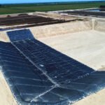
If you are responsible for the daily operation of a heap leach pad, the overliner cannot just be judged by whether it has been “laid down”; you must look at the thickness, particle size, moisture status, spreading sequence, and vehicle traffic control. In field experience, many liner damages are not due to problems with the membrane material itself, but because the overlying protective layer is locally too thin, coarse particles are concentrated, or the unloading height is too large, causing point loads on the membrane surface.
A common practice is to control the overliner thickness at 300–500 mm, set the upper limit of coarse particles according to the design gradation, keep the free fall of unloading within 1 m, and re-measure the thickness and flatness by section to avoid long-term local high pressure on the membrane surface.
Material
The first inspection of the overliner is not “has the material arrived,” but “what is in the material.” Even if labeled as a protective layer, some materials form a continuous buffer surface after spreading, while others start to segregate within 2–3 days, with coarse particles rolling forward and fine materials staying behind; sometimes metal fragments, wood chips, or hard concrete blocks get mixed in. For materials laid on top of HDPE or LLDPE liners, the site focuses more on maximum particle size, particle shape, fines ratio, moisture status, impurity content, and stratification stability. If any of these deviate from the design range, the subsequent heap load of 50–150 kPa will amplify the stress on the membrane surface.
First, look at the particle size. Many projects control the maximum particle size of the overliner at 25–50 mm, not for aesthetic reasons, but because exceeding this significantly reduces the local contact area. A 40 mm rounded particle and a 40 mm sharp-edged crushed stone exert completely different contact modes on the same membrane surface; the former is more like a distributed load, while the latter is more like point pressure. If 60–75 mm oversized rocks are mixed in, a single pass might not cause an immediate problem, but under continuous loading and temperature cycling, indentations will slowly form on the membrane. The site won’t just check if there are “big rocks,” but will look at the oversized percentage based on sieve results; many standardized practices control oversized material to within 1–3%, beyond which re-sieving or rejection is required.
Looking at the maximum particle size alone is not enough; you must also check the gradation continuity. If the protective layer is too uniform, the voids will be too large and particles will struggle to interlock; if the fines ratio is too high, drainage efficiency will drop, and it will be more prone to forming a softened layer after spraying or rain. A common field practice is to check the sieve curve against the design envelope to ensure that the passing rates for 4.75 mm, 9.5 mm, 19 mm, 25 mm, etc., fall within the allowed range. For users, this data is much more useful than “looking about right” because even if a load looks fine to the naked eye, sieving may reveal a concentration in a certain size range, leading to segregation after spreading.
The following table is suitable for site acceptance or material yard inspections:
| Inspection Item | Common Control Range | Field Focus |
|---|---|---|
| Maximum Particle Size | 25–50 mm | Whether oversized rocks are mixed in |
| Oversized Material Ratio | Within 1–3% | Whether secondary sieving is needed |
| Fines Ratio | Per design envelope | Too much causes compaction, too little causes segregation |
| Impurity Content | No visible foreign objects | Metal, wood, concrete fragments |
| Moisture Status | Spread-able, level-able | Too dry leads to segregation, too wet leads to rutting |
| Particle Shape | Rounded preferred | High ratio of sharp particles will press into the liner |
Particle shape is more important than many think. Angular particles are common in crushed ore; if used as overliner, little difference is seen during laying and initial compaction, but once the upper ore begins to be heaped, sharp particles form higher local stress at contact points. Field judgments are generally not made by “looking sharp,” but by sampling the edge-to-edge ratio; some projects spread samples in shallow trays to count the proportion of sharp particles. As long as sharp particles account for a high proportion of the coarse component, linear indentations may still appear on the membrane even if the total thickness reaches 400 mm. If there is vehicle traffic above, these indentations will continue to deepen within 7–30 days.
After controlling size and shape, fines content must be checked. Fines are not “the fewer the better.” Without enough fines, the coarse materials won’t fill in, and the spread protective layer will act like a skeleton—level on the surface but with large internal voids, prone to collapse after 10–20 passes by vehicles; too many fines make the material denser under wet conditions, slowing down moisture migration above the drainage layer and potentially causing local siltation near blind drains. The common practice is to look at sieve results and moisture status together. For example, the same fines ratio might be just spreadable at 4–6% natural moisture but show bonding and wheel track closure at 8–10%.
The impact of moisture status on spreading quality is greater than many estimate. If the material is too dry, coarse and fine particles separate faster during unloading; if too wet, it is easily squeezed into ripples by tracks or tires, forming shallow grooves of 30–60 mm. In windy and dry weather, it’s common for the surface and interior of a pile to differ by 2–4 percentage points in moisture; a sample might pass in the morning, but the material has segregated by the afternoon’s spreading. A more standard practice is to check moisture and gradation once per shift or every 500–1,000 m³, increasing to every 250–500 m³ when the material source changes rapidly.
When transitioning to impurity control, field issues become more specific. The biggest threat is not “large amounts of debris” but a small amount of high-hardness foreign objects going unnoticed. Metal strips, steel wires, wood stakes, hard plastic shards, concrete corners, and old liner weld beads can all be pressed into the membrane after spreading or rolling. Even if a foreign object is only 30–80 mm long, its irregular shape is enough to create a hard point under the overlying load. Field checks usually involve two steps: visual removal at the loading point and a walk-through by an inspector along the leading edge of the pile after unloading. This task should not rely solely on the driver or loader operator; independent records are best because many objects are exposed at the front edge only after rolling during unloading.
In addition to the material itself, source stability must be monitored. A heap leach pad often uses multiple sources: natural gravel, crushed ore, or screened material from a borrow pit. As long as the source switches within 1–2 weeks, the particle shape, moisture, and fines ratio may change. For construction and operations personnel, the most problematic situation is mixing two materials with very different properties in the same section. The first half might be rounded gravel and the second half sharp crushed stone; the thickness readings might all meet the standard, but the stress on the membrane and subsequent settlement will not be the same. Zoning records should clearly state the source ID, date of use, coverage area, and test batch so that if drainage response slows down or indentations appear, the specific batch can be traced.
The following checklist is suitable for site and entry acceptance forms:
- Assign separate IDs for each material source; do not mix them.
- Perform a sieve verification every 500–1,000 m³.
- Add a moisture and visual check whenever the source switches.
- Stack oversized rocks and foreign objects separately; do not mix them back in.
- Batches with excessive sharp particles should not enter thin coverage areas.
- Use the same source within the same section whenever possible.
- Re-check moisture status after rain or spraying.
- Re-inspect the leading edge for newly exposed foreign objects before unloading.
Material stability is also reflected in structural retention after compaction. Some materials look good during spreading but compact quickly under repeated wheel loads; others look loose initially but become more stable after leveling. Judgment shouldn’t rely only on walking or equipment trials; it’s best combined with a test plot. A common approach is to create a 100–300 m² test area, spread it to the design thickness, and have equipment pass a set number of times—e.g., 10, 20, 30 times—then measure the wheel track depth and thickness change. If the rutting reaches 40–50 mm after 20 passes, the gradation, moisture, or equipment route should be adjusted before large-scale use.
Further down, consider the matching of materials with the underlying geotextile, drainage layer, and pipeline structures. If the overliner particle size is too coarse and the underlying geotextile weight is low, particle edges are more likely to transmit stress to the membrane through local compression. Field evaluations shouldn’t look at material in isolation but within the whole profile. For example, if the design overliner thickness is only 300 mm and heavy equipment is passing above, the tolerance for particle size, shape, and impurities will be much lower; the same material might be acceptable at 500 mm but unsuitable at 300 mm.
One type of problem often occurs during material storage. Passing at entry doesn’t mean it stays that way when used. If the storage yard doesn’t have a hardened base, mud will mix into the bottom; long-term exposure to rain and sun will cause the surface and interior of the pile to vary significantly. Loaders repeatedly taking material from the same face will cause large particles to roll to the toe, leaving fines in the upper-middle part. The result is that material taken in the morning has one gradation, and material in the afternoon has another. A safer field practice is to control the pile height and retrieval method—e.g., height should not be too great, commonly controlled at 3–5 m, and retrieval should be in layers rather than continuously from a single toe.
To make field execution easier, material management can be summarized in this simple table:
| Scenario | Suggested Action | Recording Method |
|---|---|---|
| First entry of new source | Check sieve, moisture, and impurities | Create a first-piece record |
| Source switch | Re-sample a batch | Mark on the zone map |
| Resuming after rain | Re-test moisture and gradation stability | Compare with pre-rain data |
| Abnormal rutting found | Trace back to batch source and moisture | Correlate with traffic records |
| Pipe trench or toe work | Prioritize batches with stable particle size | List batch ID separately |
| Poor test plot performance | Adjust gradation or change source | Keep before/after data |
Taking the material stage a step further: at entry, don’t just write “particle size meets requirements,” but “max size ≤50 mm, oversized ≤3%“; don’t just write “moderate moisture,” but “natural moisture falls within the validated test plot range”; don’t just write “no obvious debris,” but “visual checks at loading and unloading points showed no metal, wood, or concrete blocks.” When records are this detailed, subsequent laying, traffic, inspection, and tracing have a basis, and material problems won’t be misidentified as construction issues or vice versa.
Laying
When laying the overliner, the most common field problem is not “insufficient total volume,” but uneven distribution. The design might say 300–500 mm, but in practice, it often becomes 420 mm in the middle, 260 mm at the toe, and only 180 mm near pipe trenches. The liner bears stress at the thinnest point, not the average. Trucks unloading from height, bulldozers repeatedly turning, and coarse particles rolling to low spots all create thickness variations within a 20–30 m range. Standardizing the unloading sequence, spreading direction, and measurement points is more useful than just looking at the total area.
Consider the unloading and spreading actions. Many liner indentations aren’t visible on the first day; they appear 7–30 days after the ore is heaped because particles rearrange and local point loads concentrate. A safer construction method is to unload onto an already formed protective layer, then use low ground pressure equipment to push it forward in layers, usually 150–250 mm per layer in 2–3 layers, to prevent coarse material from crashing into thin areas. Near collection pipes, toe transitions, and anchor trenches, keep the free fall within 1 m; beyond this, 25–50 mm particles separate more easily, rolling to the front and leaving an inconspicuous hard point zone.
Unloading locations also need calculated distances. Vehicles should not dump material directly onto dense weld areas, pipe penetrations, or slope corners; a 3–5 m buffer zone is usually left for equipment to push it over. The reason is simple: these spots already have geometric changes where membrane stress is more complex; adding instantaneous impact makes indentation depth harder to control. On slopes of 3H:1V or steeper, spreading should follow contour lines to prevent coarse material from rolling down; if 50–80 mm of surface segregation appears on a slope, stop the progress, recover the coarse material, add fines, and relevel before moving on.
The following controls are suitable for site job cards for quick execution by crews:
- Single layer spreading thickness: 150–250 mm
- Total thickness verification: Flat areas no less than design; local thin areas no lower than minimum allowed.
- Unloading free fall: Ideally <1 m
- Buffer distance for welds, trenches, toes: 3–5 m
- Equipment travel speed: Usually controlled at 5–8 km/h
- Stationary turning: Prohibited
- Sudden braking: Prohibited
- Heavy vehicles prohibited until overliner reaches design thickness.
After the material is laid, the next step is measuring thickness, not releasing equipment. Construction logs stating “400 mm protective layer completed” aren’t very helpful; the site needs point data. Common practice is to set a grid of 10 m × 10 m or 20 m × 20 m in flat areas, increasing density to 5 m at toes, sides of blind drains, transitions, and maintenance roads. Records must include minimum and maximum values and point distribution. Even if a zone averages 380 mm, a few points at 220 mm will become priority damage spots under vehicle rolling.
Thickness measurement methods must be unified. Many sites use steel rods or hand-dug holes; it’s fast but error-prone, especially in loose or wet material. A more reliable method combines manual probing with cross-section surveys: one cross-section every 30–50 m with at least 3–5 points, comparing results with design elevations. Near linear structures like collection pipes, measure 1–2 m laterally rather than just on the centerline, as many thin spots occur at edge overlaps.
After thickness, check flatness. The overliner surface doesn’t need to be perfectly smooth, but it must lack sharp ridges, hard bumps, or shallow grooves. If a groove reaches 50 mm depth, subsequent spraying and wheel loads will cause fines to migrate, leading to uneven thickness; if a ridge is less than 200 mm wide, overlying ore will create linear stress faster. Field checks should use a 3 m straightedge; local differences exceeding 20–30 mm usually require repair. This action is small but far easier than later excavation and re-inspection.
Next is equipment traffic control. Many thin areas are pressed out after laying, not formed during it. The ground pressure and wheel track frequency of bulldozers, loaders, and light dump trucks differ. If equipment runs 20–50 times on the same path, it will compact the loose layer, reducing a 350 mm thickness significantly in the center of the track. Sites should preset fixed paths, with widths based on equipment plus a safety margin (commonly 4–6 m); no shortcuts or stationary U-turns are allowed in thin coverage areas.
Equipment turning radii must also be managed. Both tracked and wheeled equipment push surface material to the sides during low-speed turns, forming a profile that is low in the middle and high on the sides. If rut depth exceeds 10–15% of the design thickness, traffic should stop. For example, if the design overliner is 400 mm and ruts approach 40–60 mm, you must stop to re-measure the remaining thickness rather than just adding surface material. Surface filling only masks the shape; it doesn’t restore the compacted internal structure or the original drainage conditions.
The following points are suitable for shift handovers between site inspectors:
- Routes and number of passes for current shift equipment.
- Depth and length of new wheel ruts.
- Sampled remaining thickness at the bottom of ruts.
- Whether material is piled or exposed near toes, corners, and maintenance points.
- Whether coarse particles are concentrated at the leading edge or down-slope.
- Whether backfilled areas from the previous shift have been compacted and leveled.
- Whether shallow grooves have formed after rain or spraying.
- Any abnormal settlement above blind drains or branch pipes.
Another often overlooked area: structural transitions. Where flat meets slope, main drains meet branch drains, geotextiles overlap, or around pipe sleeves, material stiffness and geometry change. Standard spreading techniques aren’t enough here. Usually, a thinner transition layer of 100–150 mm is laid first to smooth the profile before adding the regular overliner. For small-radius transitions, the proportion of manual trimming often increases because mechanical spreading leaves hard inflection points. A 30 mm local bulge at a transition point will be pressed into deeper troughs by the weight of the ore.
If maintenance excavation occurs, backfill quality is usually less stable than initial laying. The reason is simple: excavation width is often only 0.6–1.2 m, leaving little room for machinery, and backfill tends to lack proper layering. For these narrow areas, you must not only fill to design thickness but also level and re-measure the adjacent 0.5–1 m, otherwise the boundary between new and old material will create uneven stiffness. Many local settlements during operation trace back to poor backfill density or surface transition at old maintenance points.
By managing the laying stage to this level of detail, subsequent problems become much easier to diagnose. If drainage volume changes, check for compaction zones; if a toe settles, check for illegal unloading in the 3–5 m buffer; if a maintenance road needs repeated repair, check if equipment routes are overlapping long-term.
Operation Period
Once installation is complete, the state of the overliner will not remain static. Upon entering the operation period, factors such as overlying ore loading, sprinkler leaching, vehicle maintenance, diurnal temperature fluctuations, and local settlement will continuously reshape the distribution of the protective layer. While the design thickness is 300–500 mm, after 30–90 days of operation, local areas may decrease by 30–80 mm due to compaction, scouring, or backfill disturbance. If thickness non-uniformity exists early on, subsequent changes will manifest more rapidly at the toe of the slope, on both sides of blind drains, and near maintenance access roads. Site inspections must not merely check if the surface is exposed; they must integrate thickness, settlement, drainage response, and surface migration into a single set of records.
First, consider the impact of ore loading. Once the ore enters the continuous stacking phase, the protective layer no longer bears the short-term rolling of construction equipment but rather the long-term compaction of heavier loads. In many projects, when the initial ore stack height reaches 3–6 m, the internal particles of the protective layer begin to rearrange; as local stacking height increases to 8–12 m, originally loose fine-material zones are compacted, while coarse-grained zones are more likely to form hard contact points. If the operations team only inspects the surface once a month, they can easily miss early changes. A common practice is to inspect weekly during the first 30 days after a new stacking area is commissioned, and at least every two weeks during the first 90 days, keeping a close eye on the fastest-changing stages.
Following loading, settlement ensues. Settlement does not necessarily manifest as large-scale sinking; often, it is a gradual change of 5–20 mm, appearing first at expansion joints of old heap leach pads, weak foundation areas, slope toe transition zones, and above blind drains. A single figure might not seem large, but if differential settlement occurs within an adjacent 5–10 m range, the overliner thickness and surface drainage gradient will be rewritten, and the fine-material migration speed will change accordingly. On-site settlement points are often laid out by zone, with a spacing of 20–30 m in flat areas and increased density to 5–10 m in transition zones and slope toes. As long as the difference between two consecutive readings is significantly large, one must investigate whether there is local compaction or disturbance of the underlying structure.
Settlement and thickness changes must be viewed together. In many zones, the surface remains completely covered, but the internal thickness has dropped near the lower design limit. Spot checks during the operation period do not require the high-density layout used during construction, but they cannot be omitted entirely. A standard approach is: perform spot checks at 30 days, 60 days, and 90 days for newly commissioned zones, followed by quarterly reviews; frequency should be increased at slope toes, pipeline turning points, maintenance backfill areas, and vehicle paths. Spot check points are usually deployed along cross-sections, with 3–5 points measured per section at 10–20 m intervals. If the thickness at a certain point decreases by 10–15% compared to initial records, it is no longer just observed; an evaluation for material replenishment, leveling, or traffic restriction is required.
Next comes material migration caused by leaching. During the operation period, leaching does not fall uniformly on every square meter; on-site distribution is often affected by nozzle flow rate, atomization state, pressure fluctuations, and wind direction. If one area receives higher seepage input than others over a long period, surface fines are more likely to move, first appearing as 10–30 mm shallow rills or pits, then gradually evolving into coarse-grained concentration zones. It looks like a minor issue, but once fines are migrated away from the top of the overliner, the support state between lower coarse particles deteriorates. When vehicle maintenance or local stacking load changes are added, compaction occurs faster. During the stable operation phase of leaching, it is generally recommended to check surface integrity monthly, with increased inspections during windy seasons or after nozzle adjustments.
The following set of operational observation points is suitable for a standardized inspection checklist:
- Whether shallow rills or pits of 10–30 mm have appeared on the surface
- Whether coarse particles are accumulating at the leading edge, slope toe, or leaching concentration zones
- Whether there is linear subsidence above blind drains, branch pipes, or main pipes
- Whether maintenance access backfill areas are more than 20 mm lower than the surroundings
- Whether equipment path tire tracks repeatedly fall in the same strip area
- Whether there are scouring rings or local mudding around nozzles
- Whether new water flow paths have formed after rain
- Whether local areas are close to exposure or show signs of exposed geotextile
Beyond leaching, rainfall events must be considered. Problems with the protective layer are often easier to see after moderate to heavy rain, as surface migration, edge erosion, and rill development become clearer within 24–48 hours. If a single rainfall event in the area reaches 20–50 mm, the slope toe, drainage diversion areas, and maintenance backfill zones are more prone to issues. If superimposed with a shutdown or resumption of leaching, existing drainage paths may also change. Post-event inspections usually look not only for ponding but also for new gullies along the slope, edge deformation along collection facilities, and comparisons with photos from the previous sunny-day inspection.
After several months of operation, disturbances caused by maintenance activities will gradually increase. Whenever collection pipes, leaching pipes, instrument wells, monitoring points, or valve areas are excavated, the local overliner state is rewritten. Backfill width is sometimes only 0.6–1.2 m; with small construction space, insufficient layering and poor boundary smoothing are common. The operations team must not only confirm that it is “backfilled” but also verify the thickness, surface smoothness, and transition within the adjacent 0.5–1 m range after backfilling. If re-settlement occurs in the backfill area within 24–72 hours, it indicates internal rearrangement is still ongoing, and repeated traffic should not be restored immediately.
The following table can be used to schedule operation period inspection frequency and content:
| Operation Scenario | Recommended Frequency | Priority Inspection Content |
|---|---|---|
| First 30 days of new zone | Weekly | Settlement, thickness spot checks, rills, tire tracks |
| First 30–90 days | Every two weeks | Leaching impact, surface migration, slope toe changes |
| Stable Operation Period | Monthly | Scouring, maintenance areas, equipment paths, drainage response |
| After single heavy rain | Within 24–48 hours | New gullies, edge erosion, local subsidence |
| After maintenance backfill | Within 24–72 hours | Backfill thickness, smoothing, re-settlement |
| During abnormal drainage | As soon as possible post-event | Comparison of zone records, check for compaction and clogging signs |
During the operation period, the overliner state should also be analyzed in conjunction with drainage performance. The protective layer itself is not a drainage layer, but it affects the stress and particle migration between the overlying ore and the underlying drainage structure. Once fines in a zone migrate downward or local compaction occurs, seepage paths and drainage response times may change. On-site judgment is not based solely on single-day drainage volume but on a comparison of solution input, leaching duration, historical curves for the same zone, and the performance of adjacent zones. For example, if drainage response in a zone is delayed by several hours to 1 day while input conditions remain relatively stable, and shallow subsidence or coarse-grain concentration appears near the slope toe, it is necessary to include the overliner state in the troubleshooting list rather than focusing only on the pipelines themselves.
To make problems easier to detect, many operations teams include several indicators in the same weekly report: settlement readings, thickness spot checks, tire track depths, surface photos of leaching areas, and drainage curves. Looking at single indicators in isolation often makes it difficult to find connections; once placed together, patterns become much clearer. For instance, if tire tracks in a path increase from 20 mm to 45 mm, drainage response slows down in the same week, and inspection photos show intensified fine migration near nozzles, it should not be treated as simple surface irregularity. Operation management focuses more on trends rather than whether a limit is exceeded in a single instance.
In operational records, the most useful entry is not “inspected and normal,” but “which point, how much it changed compared to last time, where it changed, and what else changed simultaneously nearby.”
In addition to walking inspections, image comparison is very practical. If photos from fixed points are taken at the same angle, distance, and time of day, changes over 2–4 weeks become easy to see, especially surface color differences, coarse-grain exposure zones, gully lengths, and sinking edges of maintenance areas. For long slopes or large flat areas, many sites take a set of photos along a fixed route, keeping 3–6 standard observation points for each zone. This is not complicated but is more reliable than relying solely on verbal impressions from the field. If combined with a simple measuring ruler, photos can change from “looks like there’s a change” to “rill increased from 12 mm to 28 mm.”
The following set of record items is suitable for permanent filing and will be used for subsequent look-backs:
- Zone number, commissioning date, initial thickness record
- Each settlement reading and coordinate of measuring points
- Difference between thickness spot check results and initial values
- Inspection photos after rain and after leaching adjustments
- Tire track depth and equipment traffic count
- Maintenance excavation location, backfill date, and restoration scope
- Time of abnormal drainage and corresponding operating conditions
- Locations and quantities of material replenishment or leveling performed
If abnormalities are found during the operation period, the processing sequence must be clear. First, determine if the problem is caused by surface migration, internal compaction, local settlement, or maintenance backfill, then decide whether to replenish material, level the surface, restrict equipment, or perform further testing. Simply replenishing the surface without investigating the cause will often lead to a reoccurrence in the same spot after 1–2 weeks. If thickness reduction, deepening tire tracks, or rill growth appear in two consecutive inspections in a certain area, it should no longer be treated as routine maintenance, but listed as a key observation zone for tracking for at least 2–4 cycles.
Monitor LDR
LDR (Leak Detection and Recovery) should not just look at “whether there is liquid,” but at the 24-hour drainage volume, 7-day average, unit area conversion values, recession time after rain, and zonal differences. In actual management, many problems do not appear on the heap surface first, but on the LDR record sheet: a certain branch line rises for 3 consecutive days, a certain pond section’s drainage recession slows down, or a quarterly baseline shifts upward overall.
Standardized Parameters
The most common problem with LDR daily reports is not a lack of data, but inconsistent parameters. Some look at the total daily discharge volume, some at instantaneous flow, some at the cumulative value during pump operation hours, and others compare rainy days with sunny days in the same row. Once the parameters change, yesterday’s 0.8 m3/day and today’s 0.8 m3/day may not mean the same thing. In the EPA technical framework for double liners and leak detection systems, action leakage rates are set based on unified units; a common notation is gal/acre/day, not “it feels like more than yesterday.” For landfills and waste piles, the action values visible in regulatory contexts are often set at 100 gal/acre/day, while the system detection capability can be as low as the 0.1–1 gal/acre/day range.
If Shift A records flow based on pump run time and Shift B records discharge based on calendar day accumulation, a 7-day curve will look “high and low,” when in reality, it is just inconsistent recording parameters.
Fix the units first. The site should maintain at least three sets of numbers simultaneously: m3/day, L/ha/day, and gal/acre/day. m3/day is suitable for station daily reports, while L/ha/day and gal/acre/day are suitable for sub-sector comparisons and referencing technical documents. Take a common error: one sector has an area of 0.8 acre with a daily discharge of 80 gal/day; another sector with an area of 2.4 acres has a discharge of 120 gal/day. Looking at the total volume, the latter is higher; after conversion, the former is 100 gal/acre/day while the latter is only 50 gal/acre/day. Without conversion, the troubleshooting priority would be reversed.
Once parameters are fixed, the second step is not to set an alarm immediately, but to establish a baseline. The baseline should cover at least 30 consecutive days, or more reliably 60–90 days, provided there are no major changes in the irrigation system, heap height, ore type, or seasonal conditions during this period. If the average discharge of a branch line over the past 30 days is 0.55 m3/day and the standard operating range falls between 0.40–0.70 m3/day, then an “anomaly” should not be written as “exceeding 1 m3/day.” Instead, it should be split into three tiers: exceeding the 30-day average by 20%, 30%, and 50%. For a low-baseline area, 0.9 m3/day is already a significant deviation; for a high-baseline area, 0.9 m3/day might still be within the normal range.
Absolute values are suitable for site-wide alarms, while relative deviations are suitable for sub-sector interpretation. By writing them separately, the daily report will not confuse small sectors with large ones.
In addition to averages, the duration of an anomaly must be fixed. A single-day rise is usually insufficient. Common management parameters include:
- A single day exceeding the 30-day average by 20%–30% is recorded for observation;
- Exceeding the 30-day average by 30% for 3 consecutive days triggers a review;
- Staying above the baseline for 7 consecutive days without corresponding rainfall, irrigation, or pump-stop explanations triggers a field investigation.
Writing it this way is more actionable than just “watching the trend.” For example, if a branch baseline is 0.6 m3/day, and it hits 0.78 on Monday, 0.81 on Tuesday, and 0.84 on Wednesday, it has been approx. 30% higher for 3 consecutive days; if it reaches 0.86 on Thursday while the rainfall record remains 0 mm, irrigation intensity is unchanged, and pump operating hours are stable, it can no longer be classified as a random fluctuation.
Further down, “anomalies” should be broken into categories rather than just using one word. Using at least four categories is more practical: Numerical Anomaly, Temporal Anomaly, Spatial Anomaly, and Instrument Anomaly. Numerical anomalies refer to daily or 7-day averages exceeding thresholds; temporal anomalies refer to levels not dropping 48–72 hours after rain stops, or rising at fixed times every day; spatial anomalies refer to only one branch line staying high within the same cell, or the gap between two adjacent branch lines exceeding 2x for a long period; instrument anomalies refer to low flow but liquid levels rising 150–300 mm within 12 hours, or a one-time surge after a long period of zero flow.
| Parameter Item | Suggested Wording | Field Use |
|---|---|---|
| Statistical Unit | m3/day, L/ha/day, gal/acre/day | Unified daily report and sub-sector comparison |
| Time Window | 24-hour value, 7-day average, 30-day baseline | Distinguishing single-day changes from sustained rises |
| Deviation Threshold | +20%, +30%, +50% | Graded response |
| Duration Condition | 1 day, 3 days, 7 days | Avoiding misjudgment from single data points |
| Spatial Condition | Single branch, adjacent branches, entire area | Determining if the problem is local |
| Event Verification | Rainfall, Irrigation, Pump Stop, Ore Loading | Providing explanations for anomalies |
With categories in place, daily report fields must be tightened. Many sites only record “discharge volume” and “remarks,” which is not enough. A more appropriate header should have at least 10 columns: Date, Branch ID, 24-hour discharge, 7-day average, 30-day baseline, discharge per unit area, rainfall in the previous 24 hours, irrigation intensity, pump operating hours, and collection sump level change. If spatial precision can be drilled down to benches or cells, add a “Working Area Location” column. If any two columns are missing, anomaly explanations become vague.
“It was high today” is not a record; “Today was 1.1 m3/day, 57% higher than the 30-day average of 0.7, 0 mm rainfall in the last 24 hours, irrigation intensity unchanged at 6 L/m2·h, liquid level rose by 220 mm” is a verifiable record.
Do not set only one threshold for unit area. In small area sectors, instrument errors and short-term drainage changes are more likely to pull the numbers high; in large area sectors, a rise in total volume might drown out small-scale local issues. Therefore, the safest method is “double thresholds”: one for absolute value and one for relative deviation. For example, the station sets the observation line for a certain type of cell at 20 gal/acre/day and the review line at 40 gal/acre/day, while also adding “3 consecutive days exceeding the 30-day average by 30%.” This way, even if a small sector only hits 18 gal/acre/day today, if its baseline was originally only 8 gal/acre/day, hitting 18 for 3 consecutive days will be caught by the system.
Look at temporal resolution. If only daily cumulative values are kept, many anomalies will be averaged out. A better practice is to keep 1-hour or 4-hour data for important branch lines while maintaining the daily report. The reason is simple: some problems aren’t “high all day,” but rise within a fixed operating window every day. For example, if the pump starts and stops frequently with fluctuating flow between 15:00 and 19:00, it might correspond to solution switching or local liquid release; whereas a steady high flow all day is more like continuous inflow. Daily accumulation writes these two different situations as the same number, making explanation much harder.
Spatial standardized parameters must also be clear. Don’t just compare “this area is higher than that area,” but specify the comparison sequence: first compare against the same branch over the past 30 days, then against adjacent branches in the same cell, and finally against the entire site average. This is because cross-area comparisons are most easily affected by area, heap height, irrigation coverage, and drainage paths. A common judgment rule: if a branch line is 1.5–2.0x higher than its adjacent branch for 7 consecutive days, despite similar 24-hour rainfall and identical irrigation records, it should be listed as a specific target for field investigation rather than being lumped into “entire site generally normal.”
Compare with self first, then with adjacent areas, and finally with the whole site. If the sequence is reversed, local issues are often covered by the total volume.
Standardized parameters must also distinguish between “explainable anomalies” and “unexplainable anomalies.” Explainable anomalies mean a corresponding event can be found in the same table, such as 22 mm of rainfall in the past 24 hours, a 25% increase in irrigation, or pump recovery after a 3-hour stop; unexplainable anomalies mean discharge rose but no matching event is in the table. Both must be recorded, but with different processing levels. The former enters observation; the latter enters review. If unexplainable anomalies appear 2 consecutive times, even if they don’t exceed absolute alarm lines, they should trigger branch inspections, level checks, and meter calibrations.
Once the parameters are set, do not change them frequently in monthly reports. Changing from calendar day today to shifts tomorrow, or total volume this month to area conversion next month, breaks the trend line. A better approach is to keep the raw data while writing the rules into a fixed template, executing it for at least 90 days before evaluating if adjustments are needed.
Operating Conditions
Looking at LDR daily reports in isolation makes it easy to mistake normal process changes for liner issues, or to dismiss multi-day anomalies as “weather effects.” A safer practice is to put discharge volume, irrigation volume, rainfall, heap height changes, working location, level records, and pump downtime on the same timeline. For instance, if an LDR in a certain sector rises from 0.5 m3/day to 1.2 m3/day, that alone doesn’t prove a problem; first check if there was 15–30 mm of rain in the past 24–72 hours, if irrigation intensity was adjusted from 6 L/m2·h to 8 L/m2·h, or if new ore was just placed in that area.
The same LDR curve has completely different explanations in two scenarios: “irrigation increased by 20%” vs. “irrigation unchanged.” The former checks for increased inflow first, while the latter checks for local ingress, blocked drainage, or meter deviation.
Fix the time granularity first. Most sites record by shift, but the most suitable values for judgment are 24-hour cumulative value + 7-day rolling average + 30-day baseline. The 24-hour value is used for short-term changes, the 7-day average suppresses single-day noise, and the 30-day baseline determines if the overall level has risen. A simple interpretation parameter: if a branch average was 0.6 m3/day over the last 30 days (typical range 0.4–0.8 m3/day) and it stays above 1.0 m3/day for 3 consecutive days, it is already approx. 67% higher than the average and can no longer be treated as “random error.” If the 7-day average also rises from 0.6 to 0.9 m3/day, it indicates it’s not an isolated one-day event, but that continuous inflow or discharge conditions have changed.
To make data comparable, convert total discharge into discharge per unit area. The EPA frequently uses gal/acre/day in the double liner/leak detection framework to express action leakage rates. Typical regulatory action values can be found at 100 gal/acre/day, while system detection sensitivity can be as low as the 0.1–1 gal/acre/day range. Site management doesn’t necessarily have to copy the same threshold, but the unit area parameter is useful: Area A is 2 acres with 40 gal/day discharge, Area B is 0.5 acres with 20 gal/day discharge. By total volume, Area A is higher; after conversion, Area A is 20 gal/acre/day while Area B is 40 gal/acre/day. The one that truly needs checking first is Area B.
Without area conversion, comparison between sub-sectors is almost impossible. Area, heap height, and irrigation coverage all vary; looking only at “how many cubic meters today” is misleading.
Rainfall should be pulled out separately and not just viewed for the current day. A common situation in heap leach pads is that LDR rises within 6–24 hours after rainfall and gradually recedes within 24–72 hours; if the drainage layer is clear and surface drainage is normal, the recession is usually fast. Conversely, if a certain area remains high two days after rain stops, or if the whole site recedes while a single area does not, suspect local drainage blockage, low-point pooling, ingress at slope junctions, or long-term liquid retention in a sector above the liner. In actual records, it’s best to keep hourly or 6-hourly rainfall rather than just “rainy.” The same 20 mm of rain has a different impact on surface infiltration and short-term drainage pressure if it’s concentrated in 2 hours versus spread over 18 hours.
Irrigation records shouldn’t just say “on” or “off.” At least four items are most useful for LDR interpretation: irrigation intensity, irrigation duration, total irrigation volume, and irrigation area location. For example, if a day shift on a certain bench raises irrigation from 5 L/m2·h to 7 L/m2·h for 10 hours, based on a 10,000 m2 irrigation area, the increase in inflow for that shift is 200 m3; whether this reflects in the LDR depends on heap moisture status, drainage layer conditions, surface runoff, and recovery system configuration. If the LDR only increases by 0.2 m3/day, it usually doesn’t support “simple irrigation increase leading to significant bottom inflow”; if it increases by 0.8–1.0 m3/day for two or three consecutive days and is concentrated in the same sector, it is more likely a local channel, low-point pooling, or restricted drainage layer rather than just a normal irrigation response.
The item most likely missing from field tables is “irrigation area location.” Without the location, readers only know total inflow changed, but not which bench it was.
Heap height changes should also be in the same table. Public materials from SRK regarding heap leach pad design and operation mention multiple times that ore characteristics, heap pressure, moisture status, and drainage conditions together affect pad and discharge performance. For every 2–5 m increase in heap height, bottom contact stress and local fines compaction can change; if a new layer was just completed in a certain phase and the local fines content is high, the drainage path above the drainage layer may slow down. The LDR might not show “more liquid coming in,” but rather “liquid that could have drained quickly is now staying longer.” Therefore, the daily report should add two columns: Current Heap Height Range and New Layer Placement/Leveling/Frequent Vehicle Traffic in the last 7 days.
Ore particle size and fines ratio also affect interpretation. Suppose you started processing a batch of ore with a higher fines ratio two weeks ago; on the surface, total irrigation is unchanged and rain is minimal, but the internal seepage path, moisture retention, and local saturation zone formation conditions have changed. Many “slow-rise” LDRs appear in this situation: not a sudden jump on one day, but a gradual rise from 0.5, 0.6, 0.7 to 1.0 m3/day over 10–14 days. Encountering this curve, you usually won’t find the cause by checking just today’s events. It is more useful to look back at ore source, size distribution, stacking location, and heap leveling records from the past two weeks, and then check if the 7-day average for that sector has moved up synchronously.
Pump and sump records should also be viewed side-by-side. If the LDR flow meter shows low flow, but the collection sump level rises by 150–300 mm in 12 hours, or the pump start/stop frequency increases from 6 to 15 times a day, it means “there is liquid in the system,” but the measurement point is not fully reflecting it. Conversely, if flow suddenly rises while the level is not high, and it happens to be after a pump recovery, it might just be short-term accumulated liquid being pumped out at once, and doesn’t represent a significant increase in actual daily inflow. Adding level change, pump operating hours, and abnormal downtime to the daily report makes many “unintelligible peaks” easy to explain.
In a single day, flow, level, and pump start/stop should match at least two out of three. When only a single number remains, misjudgments increase significantly.
Also look at sub-sector differences rather than just site-wide totals. The site-wide LDR rises from 3.8 m3/day to 4.4 m3/day, seemingly only 0.6 m3/day more; but if broken down, you find five sub-sectors are stable while one rose from 0.3 to 0.9 m3/day, the troubleshooting priority changes completely. Sub-sector data should be fixed to branches, cells, or benches, not just “large areas.” For small, clearly located segments, even a fixed rise of 0.2–0.3 m3 every afternoon for 3 consecutive days might be more indicative than a 1 m3 site-wide increase, because it points to a specific location rather than a site-wide common influence.
For temporal bridging, it is recommended to look at at least 5 days in an “Before–During–After event” sequence. For example, if there is 22 mm of rain on Tuesday, irrigation is halved on Wednesday, and returns to normal on Thursday; put the LDR for Monday through Friday in one row. If it rises on Tuesday, stays high on Wednesday, and recedes on Thursday, it looks more like weather and short-term retention; if it stays high on Thursday and Friday, and only in the Southwest corner branch, it no longer looks like a short-term weather response. Many misjudgments come from only clipping one or two days of data, ignoring the recession trajectory after the event.
Another often overlooked item is recovery solution balance. If irrigation inflow increases by 80 m3/day, recovery solution increases by 75 m3/day, and LDR only increases by 0.3 m3/day, this set of data can generally explain itself; but if irrigation hasn’t significantly increased and recovery hasn’t risen, yet LDR increases by 0.7–1.0 m3/day for 5 consecutive days, you must seriously check for unrecorded inflow, local short-circuiting, slope runoff, or if a segment of LDR measurements is affected by piping state changes. Solution balance doesn’t need to be as complex as a research report; daily alignment of at least total irrigation, total recovery, and total LDR will expose many anomalies earlier.
Looking only at LDR, you see a result; putting inflow, recovery, and level together, you see the process.
Don’t set only one threshold. Rather than “alarm when an absolute value is exceeded,” it is more practical to set three conditions in parallel: absolute threshold, relative baseline deviation, and duration. For example, discharge per unit area exceeds a site-set value; or it is 30% higher than the 30-day average for 3 consecutive days; or it fails to return to the baseline 48 hours after rain stops. If two out of three are met, enter field review. This avoids two common errors: one is where a small area sector has a low absolute value but a very obvious relative deviation; the other is where a number is high for one day but drops back the next, which doesn’t support a sustained anomaly.
Protection for Exposed Areas
An exposed area is not a “gap waiting for coverage”; it must be managed itself. In public specifications, common HDPE geomembrane thicknesses cover 0.75–3.0 mm, with more demanding extreme conditions commonly seeing 1.5–3.0 mm; but thickness isn’t everything. The more common problems in exposed areas are UV, wind, temperature fluctuations, construction contact, and sharp stone crushing. Practices must fall into three categories: shortening exposure time, adding buffer layers to the membrane surface, and writing inspections and repairs into crew workflows.
Crushing & Puncture
Whether crushing and puncture can be prevented depends not on “whether a membrane was laid,” but on whether the membrane, protection layer, overlayer, and construction path are coordinated under the same set of conditions. In public specifications, the common thickness range for HDPE geomembranes is 0.75–3.0 mm (30–120 mil); for higher performance HDPE specs, the common range starts from 1.5 mm. As thickness increases, the membrane body’s ability to withstand local stress improves slightly, but most crushing and punctures are not solved by membrane thickness alone; they mostly occur at sharp stones, concrete corners, temporary access rollers, material impact, and wrinkle overlaps.
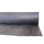
Public protection layer specs are also clear: non-woven geotextiles are used as protection layers above or below the geomembrane to mitigate punctures and tears from rock, stones, concrete, or other hard surfaces/objects. GSI’s GT12 data also gives coverage ranges for common non-woven geotextiles used for protection, with the quality range listed on public tutorial pages being 340–2000 g/m² (10–60 oz/yd²). This range already proves one thing: a protection layer isn’t just “having a cloth,” because between 340 and 2000 g/m², there is a nearly 6x difference, and the corresponding cushioning capacity will not be the same.
If the site surface is already relatively flat with a high fines ratio and only bears short-term personnel traffic, risks are usually concentrated in stones stuck in shoe soles, tool corners, and local indentations near welds; if drainage gravel, coarse ore, or precast concrete are to be placed on top, the risk shifts to point loads and corner stress. The common appearance of crushing is not a “big hole,” but starts with whitening, surface abrasions, local indentations, or slight nicks, which then turn into more obvious damage after repeated stress. ASTM D4833
From a field use perspective, identifying which types of forces are appearing on the membrane surface is more useful than vague talk about “strengthening protection”:
- Point Loads: Sharp stones, bolt heads, welding rod ends, dropped hardware; the contact surface is often only a few millimeters.
- Line Loads: Scraps, steel edges, component ridges; contact length increases, but compressive stress remains very high.
- Surface Loads: Tires, tracks, stacked material; the area is larger, but once a hard point is underneath, it still converts to a point load.
- Repetitive Loads: The same path is walked 10, 50, or 100 times; indentations accumulate.
- Material Impact: The greater the height difference, the more obvious the impact; gravel edges are more likely to pierce through weak points.
Among the above types of forces, the most commonly underestimated is “a hard point hidden under a surface load.” Tires or footsteps themselves aren’t sharp, but if a 20–40 mm angular stone is left under the membrane, contact will concentrate in a very small area. GT12 defines the protection layer as cushioning material, specifically to spread this local stress, increasing the contact area seen by the membrane and lowering the peak stress. Without a protection layer, the membrane bears a sandwich squeeze of “hard object–membrane–hard subgrade”; with a protection layer of sufficient thickness and compression performance, the load path becomes “hard object–protection layer deformation–membrane–subgrade,” and the peak force on the membrane surface will drop.
To determine if it can hold up in the field, don’t just look at a single material parameter. At least look at these items together:
- Membrane Thickness: Common HDPE specs 0.75–3.0 mm, with higher requirements often seeing 1.5–3.0 mm.
- Protection Layer Quality Range: Public tutorial pages list 340–2000 g/m².
- Overlayer Particle Size and Angularity: Rounded material acts differently than fresh gravel.
- Loading Method: Spreading from a low height vs. dumping from a high place leads to different results.
- Traffic Frequency: Crossing 3 times vs. 30 times a day leads to different cumulative indentations.
- Subgrade Condition: Smooth, without hard points, is better at reducing local crushing than a “slightly thicker membrane.”
Further, this is why many projects require constructing test pads. GSI GS11 discusses constructing test pads to evaluate whether protection materials can prevent geomembrane puncture. It’s not discussing a small test strip in a lab, but validating “membrane + protection layer + overlayer + construction method” in a simulated field setting. GS11 also specifically mentions that common protection materials are often thicker needle-punched non-wovens. The reason is practical: lab index values show material trends, but the actual result is often decided by particle grading, angularity, compaction method, and construction equipment paths.
The test pad approach is very helpful for writing as it breaks “can it hold up” into verifiable questions.
| Field Variable | Details to Confirm | Common Consequences |
|---|---|---|
| Subgrade | Presence of protruding hard points, concrete burrs, residual hardware | Membrane bottom indentations, bottom puncture |
| Protection Layer | Quality range, thickness feel, continuous coverage | Hard points not cushioned |
| Overlayer | Particle size, angularity, drop height | Top impact nicks/cuts |
| Equipment | Tire/track path, turning radius, repetition count | Local repeated crushing |
| Membrane State | Presence of wrinkles, bridging, tension whitening | Wrinkle peaks are more prone to pressure |
| Weather | Thermal expansion/contraction, surface moisture changes | Fit state changes, uneven local stress |
With the table above, determining if a protection layer is sufficient no longer requires guessing by experience. Take a common scenario: a coarse gravel drainage layer with sharp angles is to be laid over the membrane, and construction equipment will repeatedly pass over the same line. In this combo, puncture is not a single impact issue, but a superposition of “coarse angular material hard points + repeated equipment rolling.” Increasing membrane thickness alone has limited effect; moving the protection layer from a lighter grade to a higher grade is usually closer to the problem itself.
There’s another easily missed detail: puncture doesn’t only come from above the membrane; problems can also arise from below. If subgrade leveling is not clean, leaving gravel points or concrete fragments, once the overlayer load arrives, hard points will press from the bottom up. GT12’s phrasing already includes protective covering or underlayment, meaning the protection layer could be placed above or below. For slope transitions, toe of slopes, anchor trench mouths, and near penetrations, the bottom protection is often more useful than the top because the geometry varies more there, and the membrane is more prone to bridging, small wrinkles, and local stress concentrations.
From an inspection standpoint, you don’t have to wait until the end to find damage. The crew can already see many signals daily:
- Whitening, slender scratches, or dot-like indentations on the membrane surface.
- Protection layer being dragged away, exposing bare membrane strips over 50 mm or 100 mm.
- Whether regular wheel tracks or repeated dark indentations appear locally after the overlayer is spread.
- Whether polygonal pressure zones appear at slope transitions.
- Whether stones are stuck near welds, forming protrusion points.
- Whether semi-circular squeeze marks appear around pipe openings.
If indentations are already seen on-site, don’t just look for penetration. Many membrane surfaces only show dents or abrasions initially, but damage will continue to develop with subsequent temperature changes, load changes, or repeated traffic. The definitions of destructive and non-destructive assessment in GM29 indicate that the industry default is to find problems during the installation phase, not after commissioning. For exposed areas, inspection frequency should at least follow the process: once after deployment, once after protection layer placement, once before overlayer entry, and once more after heavy vehicle passage. If a sector experiences 4 nodes in a day, making 4 records is closer to the field than “inspecting once a day.”
Quantifying Re-inspections
Writing exposed area maintenance as “adjusting per weather, limiting traffic, and regular re-inspection” is not enough; field crews need to see hours, counts, ranges, and trigger conditions. In public data, common HDPE geomembrane specs cover 0.75–3.0 mm, with specs for higher performance often starting at 1.5 mm; GSI data also mentions that materials for exposed conditions include weathering assessments. Having weather-resistance requirements for the material doesn’t mean on-site exposure time can be ignored; most installation damage still occurs during deployment, waiting for coverage, cross-operations, and repeated trampling.
To turn weather into numbers, first clarify “what weather requires a stop, and what weather triggers an extra inspection.” ASTM D7865 states that geomembrane panel identification, packaging, handling, storage, and deployment should be controlled per project conditions; the code itself acknowledges that each project has different site conditions. In construction language, this means you can’t just say “depending on weather conditions.” A more practical way to write for exposed areas is to trigger by shift and event node: a minimum of 3 routine inspections per shift, with 1 event inspection added after rain, strong winds, or overnight temperature drops.
For a membrane from deployment to temporary coverage, it’s recommended not to write “complete as soon as possible,” but to change it to a time window. A more executable expression: within the same working face, the next process should be entered within 4–8 hours after a single panel is deployed; sectors uncovered for more than one shift must have edge fixation, sector numbering, surface cleaning, and photo records completed before clocking out; sectors exposed overnight must have edges, welds, and protection layer positions verified the next morning before equipment is allowed near. These numbers aren’t mandatory values from a single regulation, but a translation of ASTM handling/storage/deployment requirements into crew scheduling limits.
In weather, the thing most likely to trigger extra inspections is wind. When wind picks up, the first problems aren’t usually on the whole panel, but at edges, transitions, anchor trench mouths, and temporary protection layer overlaps. Exposed area documents can write inspection items in a fixed format: edge visual confirmation every 10–15 m; check each sector at the top and toe of the slope 1 time; whether temporary ballast bags are continuous, if the protection layer is curled, and if the exposed membrane width exceeds 50 mm. This wording makes it easier for two shifts to execute according to the same standard than “inspecting for stability.”
Rainfall triggers more than just “seeing if there’s pooling.” Three things must be checked after rain: whether the membrane surface is muddy, whether both sides of the weld are contaminated by fines, and whether the slope water flow has washed the protection layer out of place. GM29 discusses site integrity assessment, covering destructive and non-destructive testing; for exposed areas, you don’t necessarily have to do destructive sampling every time, but at least mark suspected affected sectors after rain, perform visual and continuity checks first, and then decide if more testing is needed. If rain occurs after clocking out, add 1 specific re-inspection before starting work the next day, prioritized at slope toes, transitions, around penetrations, and strips not covered last night.
The following table is suitable for the main text, and readers can follow it to modify site processes:
| Trigger Scenario | Minimum Shift Action | Recording Method |
|---|---|---|
| Normal Sunny Construction | 3 inspections: Pre-work, mid-shift, pre-clock-out | Sector ID + Time + Inspector |
| Overnight Exposure | Add 1 re-inspection before next day start | Photos of edges, welds, and protection layer |
| After Rain | Add 1 specific inspection before start | Mark mud zones, pools, and wash zones |
| After High Wind | Check edges and slopes 1 time | Record exposed width and curled positions |
| Before Equipment Entry | Check paths and turn areas 1 time | Mark allowed paths |
| Before Overlayer | Check protection layer continuity 1 time | Overlap, exposed membrane, and hard point records |
The table uses no complex terminology, so crews know when to check, what to check, and how to record it.
Traffic control must also be quantified. Much damage is not from a single crush, but from indentations formed by repeated passage over the same route. For personnel traffic, free walking on the exposed membrane can be changed to fixed walkways, with walkway widths set at 0.6–1.0 m; crew members only walk on designated strips. For equipment traffic, first draw out entry/exit directions and turning radii to avoid the same point being rolled 5, 10, or 20 times. Once traffic paths are fixed, inspection is also easier as most indentations will concentrate on a few routes.
Re-inspection before equipment entry shouldn’t just be “is the membrane there.” A more useful practice is to check the route in segments, looking every 10 m for hard points, tool debris, rocks, welding rod ends, metal parts, and concrete scraps; check the turning areas, reversing spots, and slope toes 1 extra time, as they are more prone to braking, torsion, and repeated loads. If there’s a protection layer on top, check once more if the overlap is shifted and if the exposed membrane exceeds 50 mm. For a 100 m temporary access road, this inspection forms about 10 fixed observation points, making it easier to explain during shift handovers.
Protection layers and traffic must be written together. GSI’s public catalog defines GT12 as non-woven geotextile used for protection/cushioning materials, while GS11 specifically discusses how to make test pads to evaluate if protection materials prevent puncture. In field language, this means before personnel and equipment pass, don’t just ask “can we go,” but first check if there’s a protection layer under this path, if it’s continuous, and if it’s bearing footsteps, light tools, or heavier equipment. For membrane surfaces without protection, traffic frequency must be lower; with protection, random walking still can’t be changed to unlimited traffic.
When quantifying re-inspection frequency, it’s best to use “process nodes” rather than “once a day.” A sector might experience 6 nodes in a single day: deployment, welding, temporary coverage, equipment approach, protection layer placement, and overlayer preparation. If checked only 1 time before clocking out, many indentations and contaminations will be covered by subsequent processes. A more practical arrangement: check surface and edges 1 time after deployment; check weld perimeter cleanliness and continuity 1 time after welding; check path 1 time before equipment approach; check overlap and exposed membrane 1 time after protection layer; check uncovered sectors 1 time before clocking out. Doing 4–5 node inspections in one shift is closer to the geomembrane installation site than “once in the morning and once in the evening.”
- Overnight Exposure: Check edges, welds, and protection layer positions before work the next day, then let people in.
- Work after Rain: Clean mud from the membrane surface first, then check for fines on both sides of the weld.
- After High Wind: Walk all slopes and slope tops; handle exposed membrane strips exceeding 50 mm first.
- Equipment Entry: Inspect the path every 10 m, with extra checks at turn areas.
- Repeated Route Use: Perform a route review after 5 uses, and another after 10 uses.
- Shift-end Departure: ID, photo, and record the time for uncovered sectors.
The numbers can be compressed into a more unified template: 3 routine inspections per shift + 1 post-event check + 1 path check before equipment + 1 handover check before overlayer.


Leave a reply